Fundamentals of the Analysis of Algorithm Efficiency
01. A general framework for analyzing algorithm efficiency
Two kinds of efficiency:
Time efficiency, also called time complexity, indicates how fast an algorithm in question runs.
Space efficiency, also called space complexity, refers to the amount of memory units required by the algorithm in addition to the space needed for its input and output.
Now the amount of extra space required by an algorithm is typically not of as much concern. For most problems, we can achieve much more spectacular progress in speed than in space.
02. Units for Measuring Running Time
How to measure an algorithm’s running time?
We can simply use some standard unit of time measurement-a second, or millisecond, and so on-to measure the running time of a program implementing the algorithm.
Drawbacks:
- dependence on the speed of a particular computer,
- dependence on the quality of a program implementing the algorithm and of the compiler used in generating the machine code,
- and the difficulty of clocking the actual running time of the program.
How to measure an algorithm’s running time?
One possible approach is to count the number of times the basic operation is executed.(identify the basic operation of the algorithm, and compute the number of times the basic operation is executed.)
Basic operation: the operation contributing the most to the total running time. (usually the most time-consuming operation in the algorithm’s innermost loop)
- Ex) sorting algorithms: a key comparison
- Ex) algorithms for mathematical problems: some or all of the four arithmetical operations (+, -, *, /)
Time efficiency is analyzed by determining the number of repetitions of the basic operation as a function of input size.

A difference in running times on small inputs is not what really distinguishes efficient algorithms from inefficient ones. For large values of n, it is the function’s order of growth that counts:
03. Worst-Case, Best-Case, and Average-Case Efficiencies
The worst-case efficiency
- is its efficiency for the worst-
- case input of size n, which is an input (or inputs) of size n for which the algorithm runs the longest among all possible inputs of that size
- guarantees that for any instance of size n, the running time will not exceed Cworst(n)
The best-case efficiency
- is its efficiency for the best-case case input of size n, which is an input (or inputs) of size n for which the algorithm runs the fastest among all possible inputs of that size
- The analysis of the best-case efficiency is not nearly as important as that of the worst-case efficiency. But it is not completely useless, either.
The average-case efficiency
- provides information about an algorithm’s behavior on a “typical” or “random” input
investigation of the average-case efficiency is considerably more difficult than investigation of the worst- - case and best-case efficiencies
04. Asymptotic order of growth
A way of comparing functions that ignores constant factors and small input sizes
𝚶(𝒈(𝒏))
The set of all functions with a lower or same order of growth as 𝒈(𝒏)
𝛀(𝒈(𝒏))
The set of all functions with a higher or same order of growth as 𝒈(𝒏)
𝚯(𝒈(𝒏))
The set of all functions that have the same order of growth as 𝒈(𝒏)
05. Using Limits for Comparing Orders of Growth
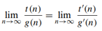
For comparing the orders of growth of two specific functions,
- A much more convenient method is based on computing the limit of the ratio of two functions
Three principal cases
- The first two cases mean that t(n) ∈ Ο(g(n))
- The last two mean that t(n) ∈ Ω (g(n))
- The second case means that t(n) ∈ Θ(g(n))
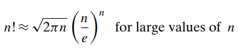
Tips : L’Hopital’s rule, Stirling’s formula
06. General Plan for Analysis Time efficiency of nonrecursive algorithms
- Decide on a parameter indicating an input’s size
- Identify algorithm’s basic operation
- Determine worst, average, and best cases for input of size n
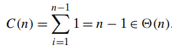
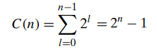
- Set up a sum expressing the number of times the basic operation is executed
- Simplify the sum using standard formulas and rules
Example 1: Maximum element
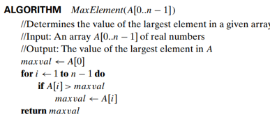
- Input size: the number of elements in the array, i.e. n
- Basic operation: comparison? assignment?
- The worst, average, and best cases?
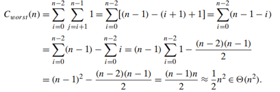
Example 2: Element uniqueness problem
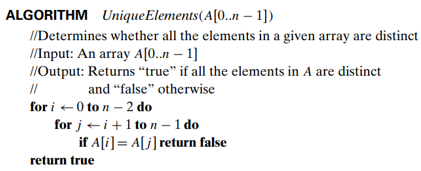
- the number of elements in the array, i.e. n
- Basic operation: comparison (in the innermost loop)
- The worst cases: (1. arrays with no equal elements 2. arrays in which the last two elements are the only pair of equal elements)
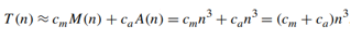
Example 3: Matrix multiplication
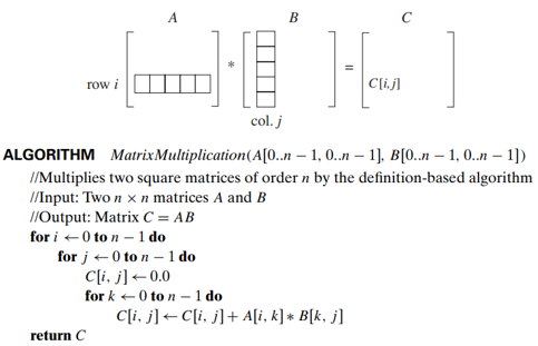
- Input size: the number of elements in the array, i.e. n
- Basic operation: multiplication and addition (on each repetition of the innermost loop each of the two is executed exactly once) : the total number of multiplications : M(n)
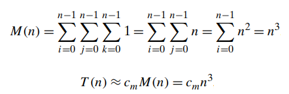
- More accurate estimation:
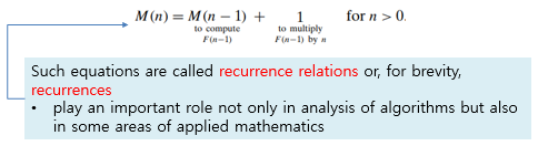
07. General Plan for Analysis Time efficiency of recursive algorithms
- Decide on a parameter indicating an input’s size.
- Identify the algorithm’s basic operation.
- Check whether the number of times the basic op. is executed can vary on different inputs of the same size. (If it can, the worst-, average-, and best-cases must be investigated separately.)
- Set up a recurrence relation with an appropriate initial condition, for the number of times the basic op. is executed.
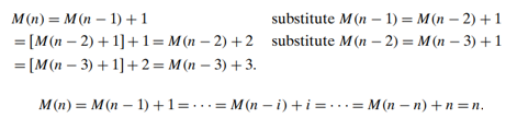
- Solve the recurrence (or, at least, establish its solution’s order of growth) by its solution (e.g. backward substitutions or another method).
Example 1: Computing factorial function
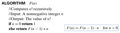
- Input size: n
- Basic operation: multiplication : the total number of multiplications : M(n)
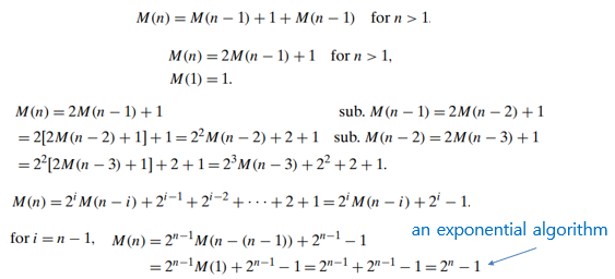
Example 2: Tower of Hanoi Puzzle
- In this puzzle, n disks of different sizes that can slide onto any of three pegs.
- The goal is to move all the disks to the third peg, using the second one as an auxiliary, if necessary
- We can move only one disk at a time, and it is forbidden to place a larger disk on top of a smaller one
- Input size: the number of disks n
- Basic operation: moving one disk : The number of moves: M(n), M(n) depends on n only
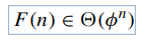
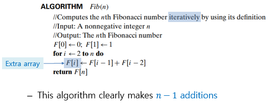
Example 3: Computing the nth Fibonacci number
Let us get an explicit formula for F(n)
- Backward substitution? : we will fail to get an easily discernible pattern
- A theorem(homogeneous second-order linear recurrence with constant coefficients, where 𝑎, 𝑏, and 𝑐 are some fixed real numbers (𝑎≠0) called the coefficients of the recurrence and 𝑥(𝑛) is the generic term of an unknown sequence to be found)
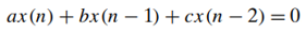
- Applying this theorem,
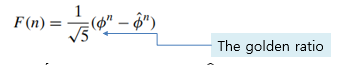
- where 𝜙 = (1 + √ 5)/2 ≈ 1.61803 and 𝜙 ̂ = −1/𝜙≈ −0.61803
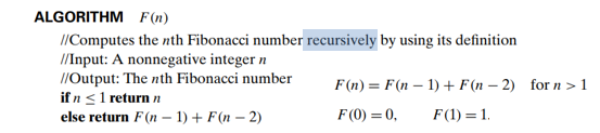
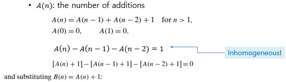
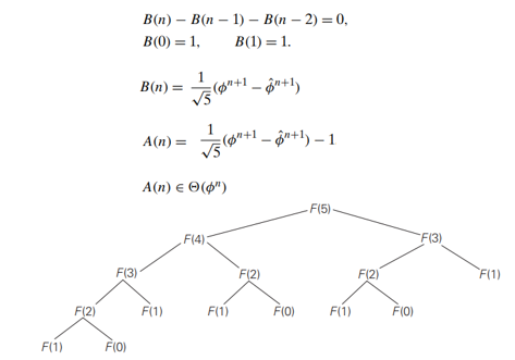
- Basic operation : addition
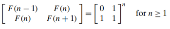
- There exists a 𝚯(log𝑛) algorithm for computing the nth Fibonacci number that manipulates only integers(an efficient way of computing matrix powers)
'학부공부 > Algorithm_알고리즘' 카테고리의 다른 글
| 05. Greedy Algorithm(1) (0) | 2021.11.18 |
|---|---|
| 04. Brute-force Search(2) (0) | 2021.11.16 |
| 03. Brute-force Search(1) (0) | 2021.11.02 |
| 01. 빅오 표기법, 시간복잡도, 공간복잡도(1) (0) | 2021.10.27 |
| 00. 알고리즘 STUDY 시작 (0) | 2021.10.27 |


댓글