Decrease-and-Conquer
01. Decrease-and-conquer technique
- is based on exploiting the relationship between a solution to a given instance of a problem and a solution to its smaller instance
- such a relationship is established, it can be exploited either top down or bottom up
- Top down > implemented recursively (ultimate implementation may well be nonrecursive)
- Bottom up > implemented iteratively (Starting with a solution to the smallest instance of the problem; incremental approach)
Three major variations of decrease-and-conquer
- Decrease by a constant (usually by 1) : the size of an instance is reduced by the same constant on each iteration of the algorithm
- Decrease by a constant factor (usually by half) : reducing a problem instance by the same constant factor on each iteration of the algorithm
- Variable-size decrease : the size-reduction pattern varies from one iteration of an algorithm to another
Decrease by a constant
The exponentiation problem of computing 𝒂^𝒏
- The relationship between a solution to an instance of size 𝑛 and an instance of size 𝑛−1 is obtained by the obvious formula : 𝒂^𝒏=𝒂^(𝒏−𝟏)∙𝒂
- Top down
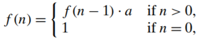
- Bottom up : By multiplying 1 by 𝑎 𝑛 times (same as the brute-force algorithm)
Decrease by a constant factor
The exponentiation problem
- If the instance of size 𝑛 is to compute 𝒂^𝒏, the instance of half its size is to compute 𝒂^(𝒏/𝟐), with the obvious relationship between the two : 𝒂^𝒏=〖(𝒂^(𝒏/𝟐))〗^2
Variable-size decrease
Euclid’s algorithm for computing the greatest common divisor
- gcd(𝑚, 𝒏) = gcd(𝒏, 𝑚 mod 𝒏) : it decreases neither by a constant nor by a constant factor
02. Decrease-by-Constant Algorithms
In the decrease-by-a-constant variation,
- the size of an instance is reduced by the same constant on each iteration of the algorithm.
- Typically, this constant is equal to one, although other constant size reductions do happen occasionally
Examples :
- Insertion sort
- Topological sorting
Insertion Sort
- To sort array A[0..n-1], sort A[0..n-2] recursively and then insert A[n-1] in its proper place among the sorted A[0..n-2]
- Though insertion sort is clearly based on a recursive idea,
- Usually implemented bottom up (iteratively)
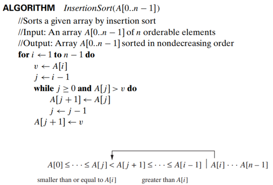
basic operation : key comparison 𝐴[𝑗]>𝑣
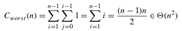
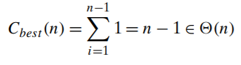
Time efficiency
the worst-case input is an array of strictly decreasing values
the best-case input is an already sorted array in nondecreasing order
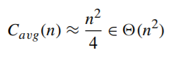
on randomly ordered arrays, insertion sort makes on average half as many comparisons as on decreasing arrays
Topological Sorting
A dag: a directed acyclic graph, i.e. a directed graph with no (directed) cycles
Applications involving prerequisite-restricted tasks : E.g. construction projects
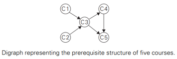
- Vertices of a dag can be linearly ordered so that for every edge its starting vertex is listed before its ending vertex
- for topological sorting to be possible, a digraph in question must be a dag
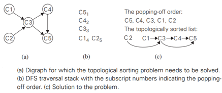
First algorithm: Depth-first search
- perform a DFS traversal and note the order in which vertices become dead-ends (i.e., popped off the traversal stack).
- Reversing this order yields a solution to the topological sorting problem
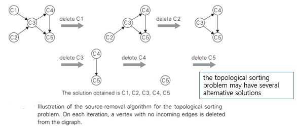
Second algorithm: Source-removal algorithm
- the decrease-(by one)-and-conquer technique
- repeatedly, identify in a remaining digraph a source, which is a vertex with no incoming edges, and delete it along with all the edges outgoing from it
- The order in which the vertices are deleted yields a solution to the topological sorting problem
03. Decrease-by-Constant-Factor Algorithms
In this variation of decrease-and-conquer, instance size is reduced by the same factor (typically, 2)
- Usually run in logarithmic time (very efficient, do not happen often)
Examples:
- Binary search
- Multiplication à la russe (Russian peasant method)
- Fake-coin puzzle
- Josephus problem
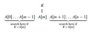
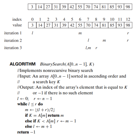
Binary Search
Binary search is a remarkably efficient algorithm for searching in a sorted array
- It works by comparing a search key 𝐾 with the array’s middle element 𝐴[𝑚].
- If they match, the algorithm stops;
- otherwise, the same operation is repeated recursively for the first half of the array if 𝐾<𝐴[𝑚], and for the second half if 𝐾>𝐴[𝑚]:
Fake-Coin Problem
Among 𝑛 identical-looking coins, one is fake.
assumes that the fake coin is known to be, say, lighter than the genuine one
With a balance scale, we can compare any two sets of coins
Idea:
- divide 𝑛 coins into two piles of ⌊𝑛/2⌋ coins each, leaving one extra coin aside if 𝑛 is odd,
- and put the two piles on the scale
- If the piles weigh the same, the coin put aside must be fake;
- otherwise, we can proceed in the same manner with the lighter pile, which must be the one with the fake coin.
a recurrence relation for the number of weighings 𝑊(𝑛) needed by this algorithm in the worst case:

Russian Peasant Multiplication
- The problem:
- Compute the product of two positive integers: 𝑛 and 𝑚
- Can be solved by a decrease-by-half algorithm based on the following formulas:
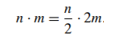
- If n is odd,
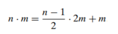
- 1 ∙ 𝑚 = 𝑚 to stop
- we can compute either recursively or iteratively
- the algorithm involves just the simple operations of halving, doubling, and adding

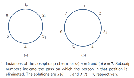
Josephus problem
- let 𝑛 people numbered 1 to 𝑛 stand in a circle. Starting the count with person number 1, we eliminate every second person until only one survivor is left.
- The problem is to determine the survivor’s number 𝐽(𝑛)
04. Variable-Size-Decrease Algorithms
the size reduction pattern varies from one iteration of the algorithm to another
Examples :
- Euclid's algorithm for computing the GCD
- Selection problem
- Interpolation search
- Searching and insertion in a binary search tree
The Selection Problem
The selection problem
- the problem of finding the 𝑘th smallest element in a list of 𝑛 numbers (the 𝑘th order statistic)
- for 𝑘=1 or 𝑘=𝑛, we can simply scan the list in question to find the smallest or largest element, respectively
- for 𝑘=⌈𝑛/2⌉, find an element that is not larger than one half of the list’s elements and not smaller than the other half (median)
Sorting-based algorithm
- we can find the 𝑘th smallest element in a list by sorting the list first and then selecting the kth element in the output of a sorting algorithm
- Efficiency (if sorted by mergesort) : Θ(𝑛𝑙𝑜𝑔𝑛)
- the problem asks not to order the entire list but just to find its 𝑘th smallest element
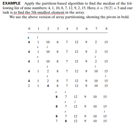
We can take advantage of the idea of partitioning a given list around some value 𝑝 of, say, its first element
- A rearrangement of the list’s elements so that the left part contains all the elements smaller than or equal to 𝑝, followed by the pivot 𝑝 itself, followed by all the elements greater than or equal to 𝑝

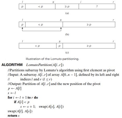
Lomuto partitioning
- a segment with elements known to be smaller than 𝑝
- the segment of elements known to be greater than or equal to 𝑝
- the segment of elements yet to be compared to 𝑝
- Note that the segments can be empty!
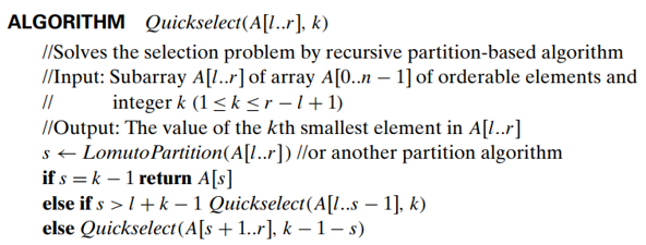
- How can we take advantage of a list partition to find the 𝑘th smallest element in it?
- Assuming that the list is indexed from 0 to 𝑛−1 : )(if 𝑠=𝑘−1, the problem is solved; pivot 𝑝 itself is the 𝑘th smallest element, if 𝑠>𝑘−1, look for the 𝑘th smallest elem. in the left part; if 𝑠<𝑘−1, look for the (𝑘−𝑠)th smallest elem. in the right part.)
- Note: The algorithm can simply continue until 𝑠=k−1.
Quickselect algorithm
- if we do not solve the problem outright, we reduce its instance to a smaller one, which can be solved by the same approach, i.e., recursively
How efficient is quickselect?
- Partitioning an 𝑛 -element array always requires 𝑛−1 key comparisons
- If it produces the split that solves the selection problem without requiring more iterations, then for this best case we obtain C_best (𝑛)= 𝑛−1 ∈ Θ(𝑛).
- In the worst case, the algorithm can produce an extremely unbalanced partition of a given array, with one part being empty and the other containing 𝑛−1 elements (e.g. 𝑘=𝑛 and an increasing array)

- the usefulness of the partition-based algorithm depends on the algorithm’s efficiency in the average case linear
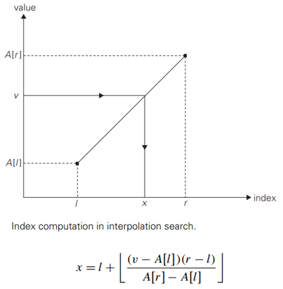
Interpolation Search
Algorithm for searching in a sorted array
- binary search always compares a search key with the middle value of a given sorted array (and hence reduces the problem’s instance size by half)
- interpolation search takes into account the value of the search key in order to find the array’s element to be compared with the search key : E.g. search for a name in a telephone book; “Brown”, “Smith”
Efficiency
- Basic operation: key comparison
- average case: 𝐶(𝑛)<log_2 log_2 n+1
- worst case: 𝐶(𝑛)=𝑛
Binary search is probably better for smaller files
Interpolation search is worth considering for large files and for applications where comparisons are particularly expensive or access costs are very high
Binary Search Tree
- Several algorithms on BST requires recursive processing of just one of its subtrees, e.g., (Searching, Insertion of a new key, Finding the smallest (or the largest) key)
- In the worst case of the binary tree search, the tree is severely skewed
- The worst-case searching : Θ(𝑛).
- The average-case searching : Θ(𝑙𝑜𝑔𝑛)
Divide-and-Conquer
01. Divide-and-Conquer
The best-known algorithm design technique:
- A problem is divided into several subproblems of the same type, ideally of about equal size
- The subproblems are solved (typically recursively)
- If necessary, the solutions to the subproblems are combined to get a solution to the original problem
- It is worth keeping in mind that the divide-and-conquer technique is ideally suited for parallel computations, in which each subproblem can be solved simultaneously by its own processor
- in the most typical case, a problem’s instance of size 𝑛 is divided into two instances of size 𝑛/2
- More generally, an instance of size 𝑛 can be divided into b instances of size 𝑛/b, with a of them needing to be solved. (Here, a and b are constants; a ≥1 and b>1.)
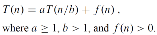
- The general divide-and-conquer recurrence : 𝑇(𝑛) = 𝑎𝑇(𝑛/𝑏) + 𝑓(𝑛) : where 𝑓(𝑛) is a function that accounts for the time spent on dividing an instance of size 𝑛 into instances of size 𝑛/𝑏 and combining their solutions.
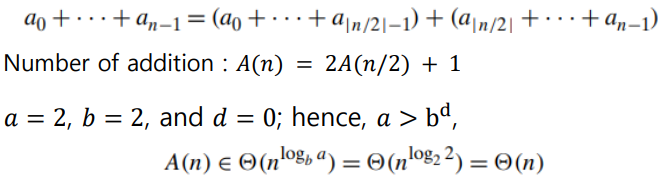
The divide-and-conquer sum-computation algorithm
Examples :
- Sorting: mergesort and quicksort
- Binary tree traversals
- Multiplication of large integers
- Strassen’s matrix multiplication
- Closest-pair and convex-hull problems
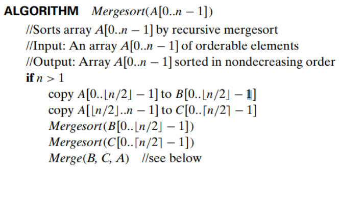
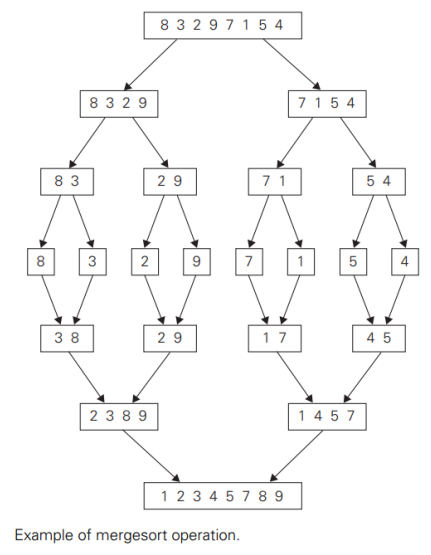
02. Mergesort
Mergesort is a perfect example of a successful application of the divide-and-conquer technique.
- It sorts a given array 𝐴[0. . 𝑛 − 1] by dividing it into two halves 𝐴[0. . 𝑛/2 − 1] and 𝐴[ 𝑛/2 . . 𝑛 − 1],
- sorting each of them recursively,
- and then merging the two smaller sorted arrays into a single sorted one
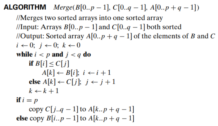
Merging of two sorted arrays :
- Two pointers (array indices) are initialized to point to the first elements of the arrays being merged. \
- The elements pointed to are compared, and the smaller of them is added to a new array being constructed;
- after that, the index of the smaller element is incremented to point to its immediate successor in the array it was copied from.
- This operation is repeated until one of the two given arrays is exhausted,
- and then the remaining elements of the other array are copied to the end of the new array
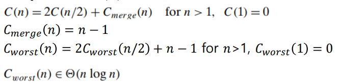
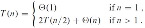
Analysis of Mergesort
- The recurrence relation for the number of key comparison 𝐶(𝑛) is
- Stable
- Space requirement: Θ(𝑛) (not in-place)
- Can be implemented without recursion (bottom-up)
- A list can be divided in more than two parts (multiway mergesort)
03. Maximum subarray problem
Example scenario
- Stock trading (When to buy and sell for maximum profit, Buying at the lowest, selling at the highest? – not always give max profit)
- Brute-force : Θ(𝑛^2)
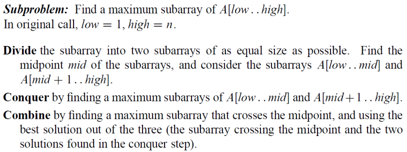
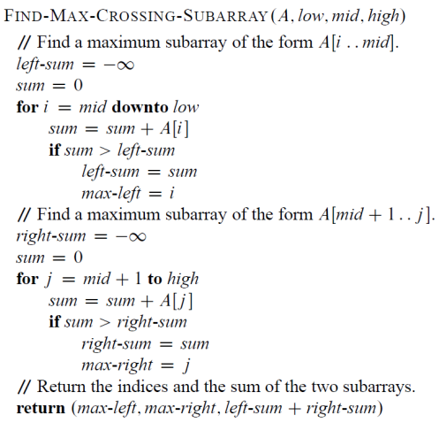
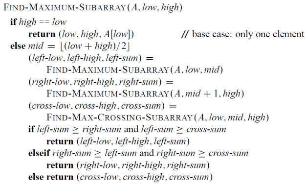
Solving by divide-and-conquer
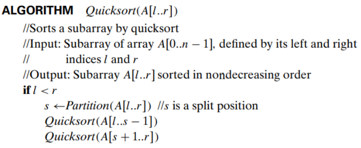
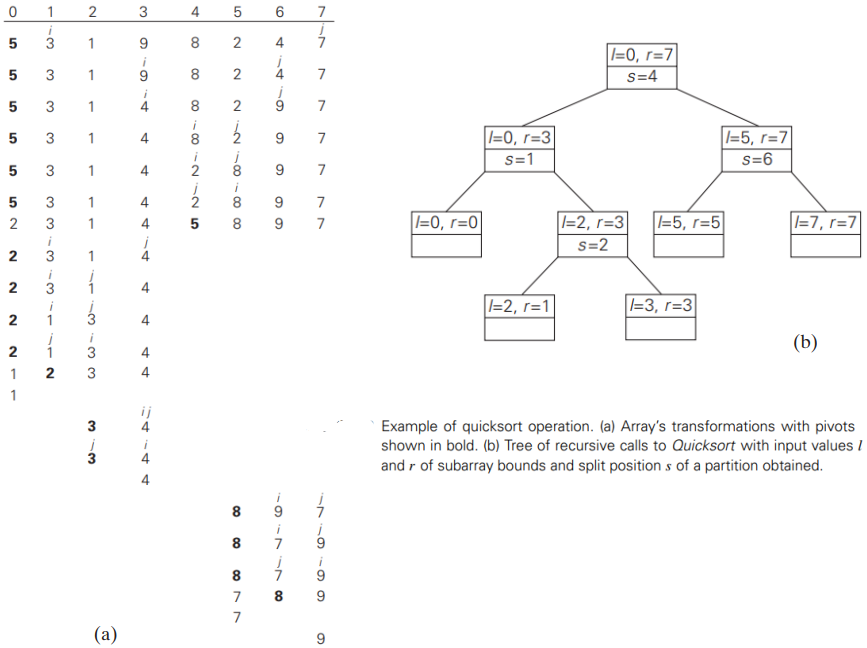
04. Quicksort
- Mergesort divides its input elements according to their position in the array
- Quicksort divides them according to their value
- Partition : an arrangement of the array’s elements so that all the elements to the left of some element A[s] are less than or equal to A[s], and all the elements to the right of A[s] are greater than or equal to it:
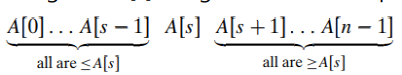
- After a partition is achieved, : A[s] will be in its final position in the sorted array, and we can continue sorting the two subarrays to the left and to the right of A[s] independently (e.g., by the same method)
- Mergesort : Division > combining (the entire work happens)
- Quicksort : Division (the entire work happens and no work required to combine)
Analysis of Quicksort
- Best case : split in the middle : Θ(𝑛𝑙𝑜𝑔𝑛)
- Worst case: already sorted array! : Θ(𝑛^2 )
- Average case: random arrays : Θ(𝑛log𝑛) : it usually runs faster than mergesort
- Improvements : better pivot selection: random element or median-of-three method that uses the median of the leftmost, rightmost, and the middle element of the array, switch to insertion sort on very small subarrays (5~15 elements), modifications of the partitioning algorithm such as the three-way partition, in combination > 20-30% improvements
- Not stable!
- selected as one of the 10 algorithms “with the greatest influence on the development and practice of science and engineering in the 20th century.”
05. Partitioning Algorithm
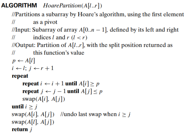
Hoare’s algorithm
- more sophisticated method suggested by C.A.R. Hoare who invented quicksort
- 1. selecting a pivot
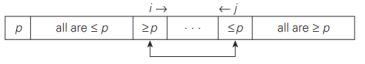
- 2. scan the subarray from both ends, comparing the subarray’s elements to the pivot
- left-to-right scan (index pointer i) : skips over elements that are smaller than the pivot and stops upon encountering the first element greater than or equal to the pivot
- right-to-left scan (index pointer j) : skips over elements that are larger than the pivot and stops on encountering the first element smaller than or equal to the pivot
- 3. After both scans stop, three situations may arise
If scanning indices i and j have not crossed, i.e., i < j, we simply exchange A[i] and A[j] and resume the scans
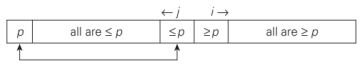
If the scanning indices have crossed over, i.e., i > j, we will have partitioned the subarray after exchanging the pivot with A[ j]:
if the scanning indices stop while pointing to the same element, i.e., i = j, the value they are pointing to must be equal to p
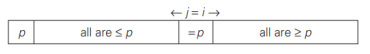
The last two cases can be combined by exchanging the pivot with A[ j] whenever i ≥ j
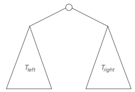
06. Binary Tree
- is defined as a finite set of nodes that is either empty or consists of a root and two disjoint binary trees 𝑇𝐿 and 𝑇𝑅 called, respectively, the left and right subtree of the root
- Since the definition itself divides a binary tree into two smaller structures of the same type : many problems about binary trees can be solved by applying the divide-and-conquer technique
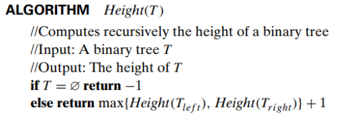
Height
- is defined as the length of the longest path from the root to a leaf.
- Hence, it can be computed as the maximum of the heights of the root’s left and right subtrees plus 1.
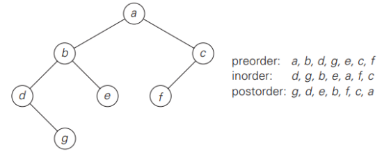
Binary Tree Traversals
- The most important divide-and-conquer algorithms for binary trees are the three classic traversals: preorder, inorder, and postorder
- All three traversals visit nodes of a binary tree recursively, i.e., by visiting the tree’s root and its left and right subtrees:
- In the preorder traversal, : the root is visited before the left and right subtrees are visited (in that order).
- In the inorder traversal, : the root is visited after visiting its left subtree but before visiting the right subtree.
- In the postorder traversal, : the root is visited after visiting the left and right subtrees (in that order).
Not all questions about binary trees require traversals of both left and right subtrees.
- For example, the search and insert operations for a binary search tree require processing only one of the two subtrees.
- not as applications of divide-and-conquer but rather as examples of the variable-size-decrease technique
07. Multiplication of Large Integers
Some applications, notably modern cryptography,
- require manipulation of integers that are over 100 decimal digits long.
- Since such integers are too long to fit in a single word of a modern computer, they require special treatment.
- This practical need supports investigations of algorithms for efficient manipulation of large integers
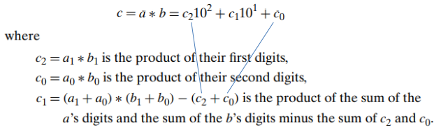
The conventional pen-and-pencil algorithm for multiplying two 𝑛-digit integers,
- each of the 𝑛 digits of the first number is multiplied by each of the 𝑛 digits of the second number for the total of n^2 digit multiplications
- For any pair of two-digit numbers 𝑎 = a_1a_0 and b = b_1b_0, their product 𝑐 can be computed by the formula
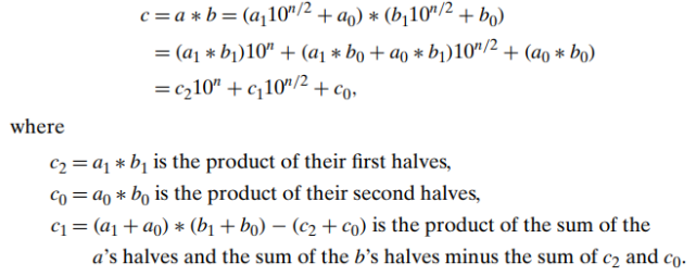
Multiplying two 𝑛-digit integers a and b (where 𝑛 is a positive even number)
- the first half of the 𝑎’s digits by a1 and the second half by a_0; for b, the notations are b_1 and b_0, respectively
- If 𝑛/2 is even, we can apply the same method for computing the products c_2, c_1, and c_0.
Thus, if 𝑛 is a power of 2, we have a recursive algorithm for computing the product of two 𝑛-digit integers.
- In its pure form, the recursion is stopped when 𝑛 becomes 1
How many digit multiplications does this algorithm make?
- Multiplication of 𝑛 -digit numbers requires three multiplications of 𝑛/2 -digit numbers
How practical is it
- On some machines, the divide-and-conquer algorithm has been reported to outperform the conventional method on numbers only 8 decimal digits long
- and to run more than twice faster with numbers over 300 decimal digits long—the area of particular importance for modern cryptography
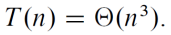
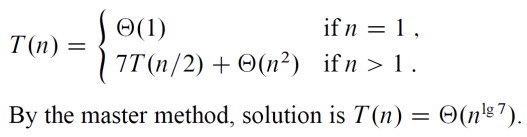
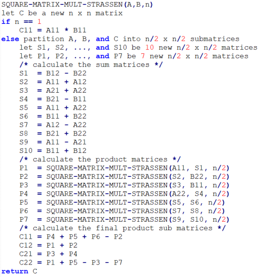
08. Strassen’s Matrix Multiplication
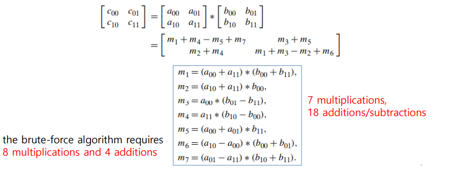
The principal insight of the algorithm lies in the discovery that we can find the product 𝐶 of two 2×2 matrices 𝐴 and B with just seven multiplications
- as opposed to the eight required by the brute-force algorithm
Let A and B be two 𝑛 × 𝑛 matrices (where 𝑛 is a power of 2)
- (If 𝑛 is not a power of 2, matrices can be padded with rows and columns of zeros.)
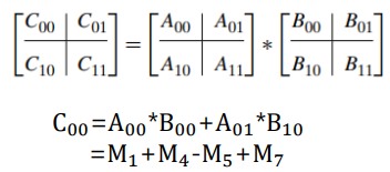
- We can divide A, B, and their product C into four 𝑛/2 × 𝑛/2 submatrices each as follows:
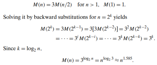
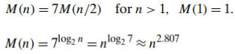
- 𝑀(𝑛) is the number of multiplications made by Strassen’s algorithm in multiplying two 𝑛 × 𝑛 matrices (where 𝑛 is a power of 2)
Since the time of Strassen’s discovery,
- several other algorithms for multiplying two 𝑛 × 𝑛 matrices of real numbers in 𝑂(𝑛^𝛼 ) time with progressively smaller constants 𝛼 have been invented
- The fastest algorithm so far is that of Coopersmith and Winograd [Coo87] with its efficiency in 𝑂(𝑛^2.376)
MatMul by divide-and-conquer
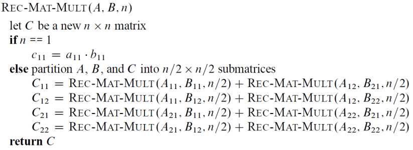
Strassen’s idea : Make less recursive, use constant # of operations instead
09. Closest-Pair Problem by Divide-and-Conquer
by brute-force algorithms in 𝚯(n^2 )
Let P be a set of 𝑛 > 1 points in the Cartesian plane
- assume that the points are distinct
- assume that the points are ordered in nondecreasing order of their 𝑥 coordinate. (If they were not, we could sort them first by an efficient sorting algorithm such as mergesort.)
- It will also be convenient to have the points sorted in a separate list in nondecreasing order of the 𝑦 coordinate; we will denote such a list Q
- If 2 ≤ 𝑛 ≤ 3, the problem can be solved by the brute-force algorithm
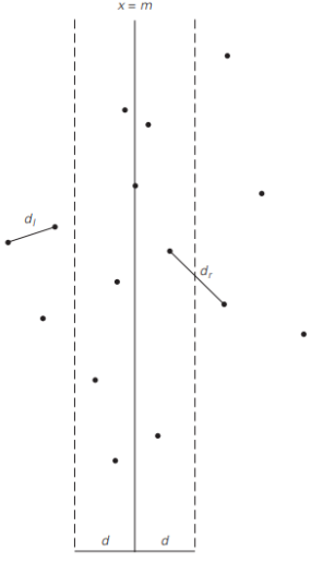
- If 𝑛 > 3, divide the points into two subsets 𝑃𝑙 and 𝑃r of [𝑛/2] and [𝑛/2] points, respectively,
- by drawing a vertical line through the median 𝑚 of their 𝑥 coordinates so that 𝑛/2 points lie to the left of or on the line itself, and 𝑛/2 points lie to the right of or on the line.
- Then we can solve the closest-pair problem recursively for subsets 𝑃𝑙 and 𝑃r .
- Let d𝑙 and dr be the smallest distances between pairs of points in 𝑃𝑙 and 𝑃r , respectively, and let 𝑑 = min{d𝑙 ,dr }.
- 𝑑 is not necessarily the smallest distance between all the point pairs because points of a closer pair can lie on the opposite sides of the separating line
- We can limit our attention to the points inside the symmetric vertical strip of width 2𝑑 around the separating line
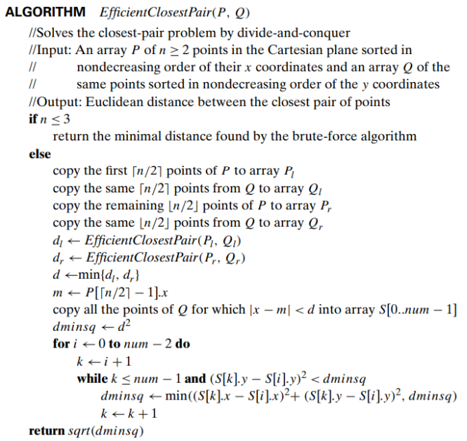
- Recurrence for the running time of the algorithm : 𝑇(𝑛) = 2𝑇(𝑛/2) + 𝑓(𝑛), where 𝑓(𝑛)∈Θ(𝑛)
- Applying the Master Theorem (with 𝑎 = 2, b = 2, and d = 1), we get 𝑇(𝑛) ∈ Θ(𝑛 log 𝑛)
- The necessity to presort input points does not change the overall efficiency class if sorting is done by a 𝑂(𝑛 log 𝑛) algorithm such as mergesort
10. Convex-Hull Problem by Divide-and-Conquer
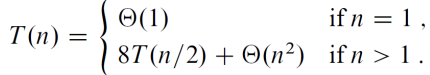
by brute-force algorithms in 𝚯(n^3 )
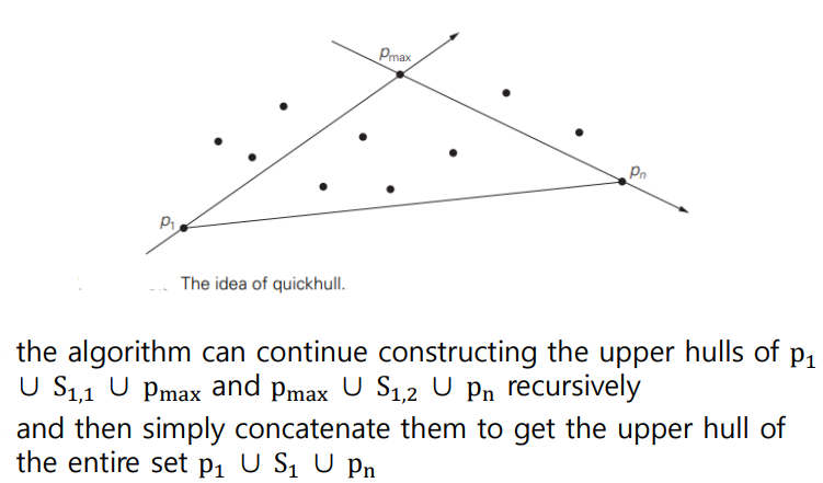
Quickhull
- a divide-and-conquer algorithm that finds the smallest convex polygon that contains n given points in the plane
- Let S be a set of 𝑛 > 1 points p1(x1, y1), . . . , pn(xn, yn) in the Cartesian plane
- the points are sorted in nondecreasing order of their 𝑥 coordinates, with ties resolved by increasing order of the 𝑦 coordinates of the points involved
- the leftmost point p1 and the rightmost point pn are two distinct extreme points of the set’s convex hull
- Let vector(p1>pn) be the straight line through points p1 and pn
- This line separates the points of S into two sets: S1 is the set of points to the left of this line, and S2 is the set of points to the right of this line
- The points of S on the line vector(p1>pn), other than p1 and pn, cannot be extreme points of the convex hull and hence are excluded from further consideration
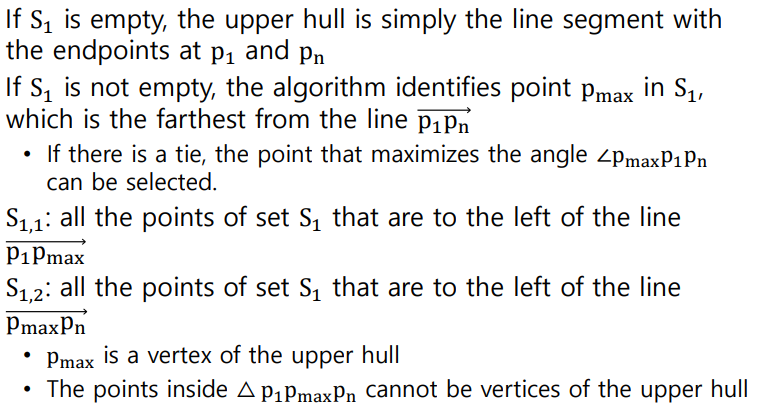
- The boundary of the convex hull of S is made up of two polygonal chains : upper hull, is a sequence of line segments with vertices at p1, some of the points in S1 (if S1 is not empty) and pn, lower hull, is a sequence of line segments with vertices at p1, some of the points in S2 (if S2 is not empty) and pn
- the convex hull of the entire set S is composed of the upper and lower hulls
How to construct the upper hull? (construct lower hull in a similar manner)
- The worst-case efficiency : 𝚯(n^2 ) (as quicksort)
- The average-case efficiency : linear [Ove80]
11. Solving Recurrences
- Substitution method
- Recursion tree method
- Master method
Substitution method
- Guess the form of the solution. > Making a good guess(Use similar recurrence, Start with loose bounds, reduce range, Use recursion trees)
- Verify by induction.
- Solve for constants
Recursion Tree
T(n) = T(n/4) + T(n/2) + n^2

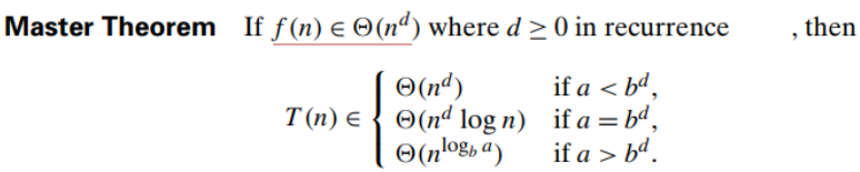
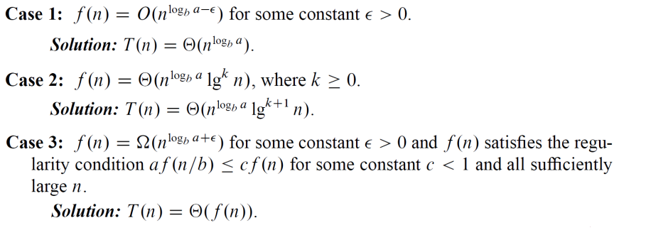
The master method
The master method applies to recurrences of the form
'학부공부 > Algorithm_알고리즘' 카테고리의 다른 글
| 10. Dynamic Programming(2) (3) | 2021.12.17 |
|---|---|
| 09. Dynamic Programming(1) (6) | 2021.12.15 |
| 07. Divide and Conquer(1) (0) | 2021.11.18 |
| 06. Greedy Algorithm(2) (0) | 2021.11.18 |
| 05. Greedy Algorithm(1) (0) | 2021.11.18 |


댓글