Greedy Technique
01. Greedy Technique
- suggests constructing a solution to an optimization problem through a sequence of steps, each expanding a partially constructed solution obtained so far, until a complete solution to the problem is reached
- On each step, the choice made must be(Feasible, i.e., it has to satisfy the problem’s constraints, locally optimal, i.e., it has to be the best local choice among all feasible choices available on that step, irrevocable, i.e., once made, it cannot be changed on subsequent steps of the algorithm)
- On each step, it suggests a “greedy” grab of the best alternative available in the hope that a sequence of locally optimal choices will yield a (globally) optimal solution to the entire problem
- From our algorithmic perspective, the question is whether such a greedy strategy works or not(there are problems for which a sequence of locally optimal choices does yield an optimal solution for every instance of the problem in question. However, there are others for which this is not the case; for such problems, a greedy algorithm can still be of value if we are interested in or have to be satisfied with an approximate solution.)
Optimal solutions:
- change making for “normal” coin denominations
- minimum spanning tree (MST)(Prim’s algorithm and Kruskal’s algorithm)
- single-source shortest paths(Dijkstra’s algorithm)
- Huffman codes
Approximations:
- traveling salesman problem (TSP)
- knapsack problem
- other combinatorial optimization problems
02. Change-Making Problem
- Given unlimited amounts of coins of denominations 𝒅_𝟏>𝒅_𝟐>...>𝒅_𝒎, give change for amount 𝑛 with the least number of coins
- Example: 𝒅_𝟏=25, 𝒅_𝟐=10, 𝒅_𝟑=5, 𝒅_𝟒=1 and 𝑛=48
- Greedy solution : 1 𝒅_𝟏, 2 𝒅_2, 3 𝒅_4 (25 + 2*10 + 3*1 = 48) This solution is optimal for any amount and “normal’’ set of denominations
- Example: 𝒅_𝟏=25, 𝒅_𝟐=10, 𝒅_𝟑=1 and 𝑛=30 : Does not yield an optimal solution
03. Minimum Spanning Tree (MST)
- Spanning tree of a connected graph 𝐺(a connected acyclic subgraph of 𝐺 that contains all the vertices)
- Minimum spanning tree of a weighted, connected graph 𝐺(a spanning tree of 𝐺 of the smallest weight)
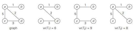
By exhaustive search
the number of spanning trees grows exponentially with the graph size (at least for dense graphs)
generating all spanning trees for a given graph is not easy
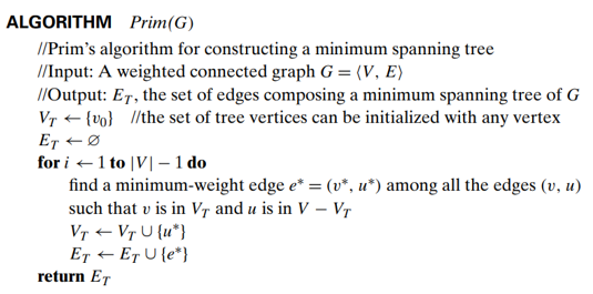
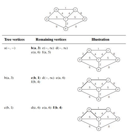
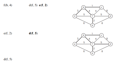
Prim’s algorithm
Prim’s algorithm constructs a minimum spanning tree through a sequence of expanding subtrees.
- The initial subtree in such a sequence consists of a single vertex selected arbitrarily from the set V of the graph’s vertices.
- On each iteration, the algorithm expands the current tree in the greedy manner by simply attaching to it the nearest vertex not in that tree.
- The algorithm stops after all the graph’s vertices have been included in the tree being constructed.
- Since the algorithm expands a tree by exactly one vertex on each of its iterations, the total number of such iterations is 𝑛−1, where 𝑛 is the number of vertices in the graph.
How efficient is Prim’s algorithm?
- The answer depends on the data structures chosen for the graph itself
- and for the priority queue of the set 𝑉−𝑉_𝑇 whose vertex priorities are the distances to the nearest tree vertices.
- if a graph is represented by its weight matrix and the priority queue is implemented as an unordered array,(the running time is in Θ(|𝑉|^2 ))
- If a graph is represented by its adjacency lists and the priority queue is implemented as a min-heap,(the running time is in 𝑂(|𝐸| log|𝑉|))
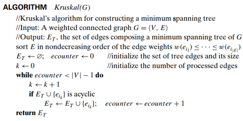
Kruskal’s algorithm
Kruskal’s algorithm looks at a minimum spanning tree of a weighted connected graph 𝐺=<𝑉,𝐸>
- as an acyclic subgraph with |𝑉|−1 edges for which the sum of the edge weights is the smallest.
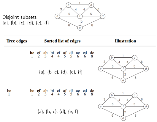
The algorithm
- begins by sorting the graph’s edges in nondecreasing order of their weights.
- Then, starting with the empty subgraph,
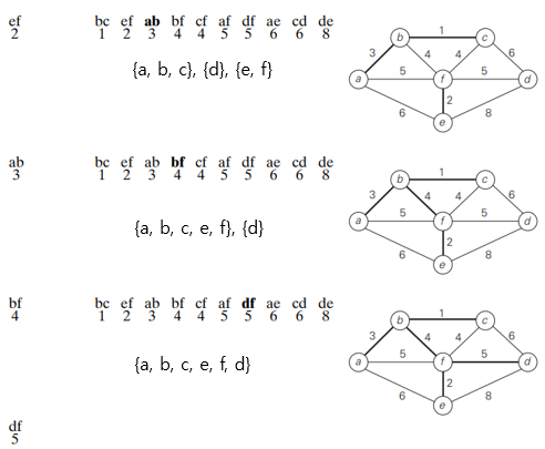
- it scans this sorted list, adding the next edge on the list to the current subgraph (if such an inclusion does not create a cycle, and simply skipping the edge otherwise.)
- Kruskal’s algorithm looks simpler than Prim’s but is harder to implement (checking for cycles!)
- Cycle checking: a cycle is created iff added edge connects vertices in the same connected component
- Union-find algorithms
- The running time of Kruskal’s algorithm will be dominated by the time needed for sorting the edge weights of a given graph.
- Hence, the time efficiency of Kruskal’s algorithm will be in 𝑂(|𝐸| log|𝐸|)
04. Minimum Spanning Tree (MST)
Shortest-paths problem
Single-source shortest-paths problem
- for a given vertex called the source in a weighted connected graph, find shortest paths to all its other vertices
- Cf. Floyd’s algorithm for the all-pairs shortest paths problem
Applications of the shortest-paths problem
- transportation planning
- packet routing in communication networks
- finding shortest paths in social networks, speech recognition, document formatting, robotics, compilers, and airline crew scheduling.
- pathfinding in video games
- finding best solutions to puzzles using their state-space graphs
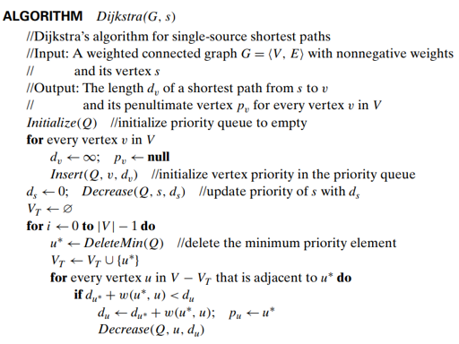
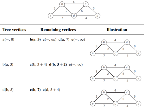
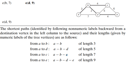
Dijkstra’s Algorithm
This algorithm is applicable to undirected and directed graphs with nonnegative weights only
First, it finds the shortest path from the source to a vertex nearest to it, then to a second nearest, and so on.
Dijkstra’s algorithm is quite similar to Prim’s algorithm
- Both of them construct an expanding subtree of vertices by selecting the next vertex from the priority queue of the remaining vertices.
- However, they solve different problems and therefore operate with priorities computed in a different manner: (Dijkstra’s algorithm compares path lengths and therefore must add edge weights, while Prim’s algorithm compares the edge weights as given)
The time efficiency
- Same as Prim’s algorithm
- depends on the data structures for representing an input graph itself
- and for implementing the priority queue
- if a graph is represented by its weight matrix and the priority queue is implemented as an unordered array,(the running time is in Θ(|𝑉|^2 ))
- If a graph is represented by its adjacency lists and the priority queue is implemented as a min-heap,(the running time is in 𝑂(|𝐸| log|𝑉|))
05. Coding Problem
Coding: assignment of some sequence of bits (codeword) to each of the text’s (alphabet) symbols
Two types of codes:
- fixed-length encoding (e.g., ASCII)
- variable-length encoding (e,g., Morse code)(frequent letters such as e (•) and a (•−) are assigned short sequences of dots and dashes , while infrequent letters such as q (−−•−) and z (−−••) have longer ones)
Prefix-free (or prefix) codes: no codeword is a prefix of another codeword
- we can simply scan a bit string until we get the first group of bits that is a codeword for some symbol, replace these bits by this symbol, and repeat this operation until the bit string’s end is reached
Huffman Trees and Codes
- If we want to create a binary prefix code for some alphabet, (it is natural to associate the alphabet’s symbols with leaves of a binary tree in which all the left edges are labeled by 0 and all the right edges are labeled by 1. The codeword of a symbol can then be obtained by recording the labels on the simple path from the root to the symbol’s leaf.)
- How can we construct a tree that would assign shorter bit strings to high-frequency symbols and longer ones to low-frequency symbols? : Huffman’s algorithm
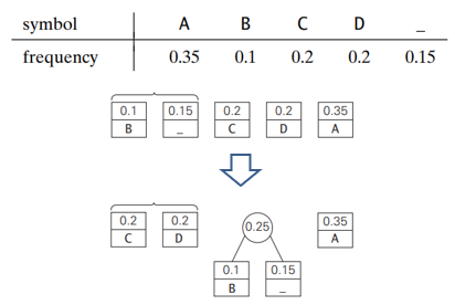
Step1
- Initialize 𝑛 one-node trees and label them with the symbols of the alphabet given.
- Record the frequency of each symbol in its tree’s root to indicate the tree’s weight. (More generally, the weight of a tree will be equal to the sum of the frequencies in the tree’s leaves.)
Step 2
- Repeat the following operation until a single tree is obtained.
- Find two trees with the smallest weight.
- Make them the left and right subtree of a new tree and record the sum of their weights in the root of the new tree as its weight.
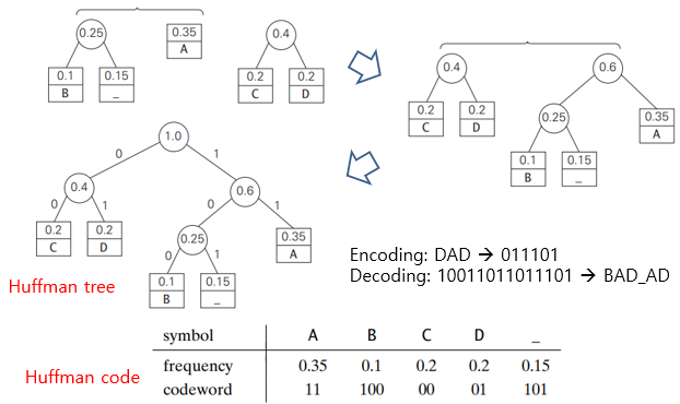
- With the occurrence frequencies given and the codeword lengths obtained, the average number of bits per symbol in this code is : 2*0.35 + 3*0.1 + 2*0.2 + 2 * 0.2 + 3*0.15 = 2.25
- Compression ratio : (3−2.25)/3×100%=25%
Activity selection problem
- The problem of scheduling several competing activities that require exclusive use of a common resource.
- n activities require exclusive use of a common resource.
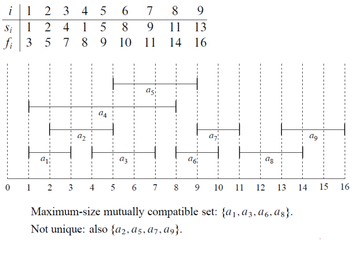
- Set of activities S={a_1 , …. , a_n }
- ai needs resource during period [s_i , f_i ), which is a half-open interval, where s_i = start time and f_i = finish time.
- Goal: Select the largest possible set of nonoverlapping (mutually compatible) activities
Example_S is sorted by finish time f_i
Optimal substructure of activity selection
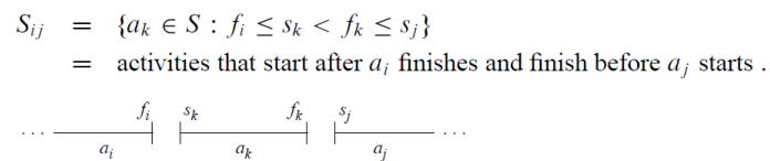
𝐴𝑖𝑗 : maximum-size set of mutually compatible activities in 𝑆𝑖𝑗
Let 𝑎𝑘 ∈ 𝐴𝑖𝑗 be some activity in 𝐴𝑖𝑗. Then we have two subproblems : Find mutually compatible activities in 𝑆𝑖𝑘, 𝑆𝑘𝑗
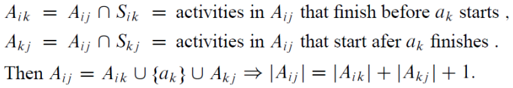
Claim : Optimal solution 𝐴𝑖𝑗 must include optimal solutions for the two subproblems for 𝑆𝑖𝑘 and 𝑆𝑘𝑗
Proof :
- 𝐴𝑘𝑗 is the optimal solution (maximum-size mutually compatible activities) for 𝑆𝑘𝑗
- Assume it is not: we can find 𝐴′ 𝑘𝑗 which is larger than 𝐴𝑘𝑗 (|𝐴′ 𝑘𝑗| > |𝐴𝑘𝑗|)
- Then |𝐴𝑖𝑘| +|𝐴′𝑘𝑗| + 1 > |𝐴𝑖𝑘| +|𝐴𝑘𝑗| + 1 = |𝐴𝑖𝑗| : contradicts!
𝑆𝑖𝑘 is symmetric
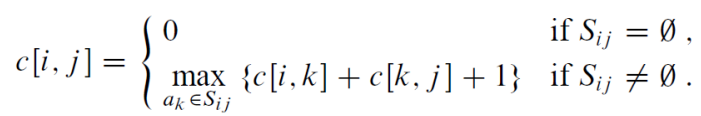
Recursive solution :
c[i, j] : size of optimal solution for 𝑆𝑖𝑗, c[i, j] = c[i, k] + c[k, j] +1
Can be solved using dynamic programming, but a greedy approach is more efficient in this case
Making the greedy choice
Choose an activity to add to optimal solution before solving subproblems
Which activity to choose?
- One leaves the resource available for the most other activities
- Answer: the activity finished the earliest(Why: remaining time is maximized, so we can assign more activities)
- Since the activity is sorted, choose a_1(Which leaves one subproblem: find a maximum size set of mutually compatible activities starting after a_1 finishes)
Is a_1 always part of optimal solution?
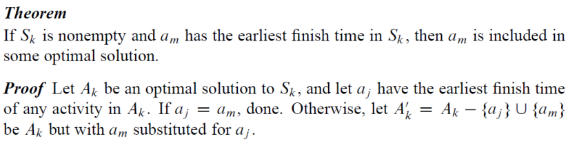
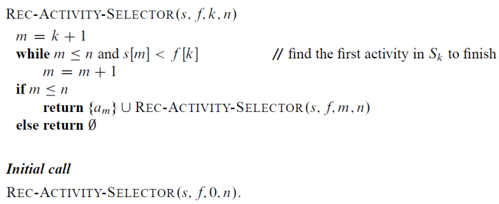
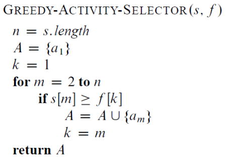
Recursive greedy algorithm
s: start, f: finish, a_0 with f_0=0, S_0=S
Key ingredients for greedy algorithm
How can we tell whether a greedy algorithm will solve a particular optimization problem?
Showing that the problem has (Greedy-choice property, and Optimal substructure)
Greedy-choice property
- Assemble a globally optimal solution by making locally optimal (greedy) choices
- Dynamic programming(Solves smaller problems first (bottom-up) : Choice depends on optimal solutions of subproblems, Memoization also requires solving smaller subproblem before larger problems using table)
- Greedy algorithms(Make the choice before solving the subproblems : Choose the currently best solution and solve the subproblem (Top-down))
How to show greedy-choice property?
- Look at an optimal solution
- If it includes the greedy choice, done
- Otherwise, modify the optimal solution to include the greedy choice and show it is just as good.
For efficiently making a greedy-choice
- Preprocess input to greedy order(e.g., activity selection – sorted based on finish time)
- Using an appropriate data structure (for dynamic case) : e.g., priority queue
Optimal substructure
- Need to show that an optimal solution to the subproblem and the greedy choice already made yield an optimal solution to the original solution
Greedy vs. Dynamic Programming
0-1 knapsack problem : Greedy method does not work
'학부공부 > Algorithm_알고리즘' 카테고리의 다른 글
| 08. Divide and Conquer(2) (14) | 2021.11.21 |
|---|---|
| 07. Divide and Conquer(1) (0) | 2021.11.18 |
| 05. Greedy Algorithm(1) (0) | 2021.11.18 |
| 04. Brute-force Search(2) (0) | 2021.11.16 |
| 03. Brute-force Search(1) (0) | 2021.11.02 |


댓글